解决问题:从蛋白质结构生成序列
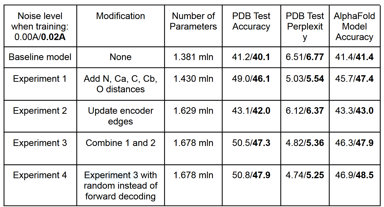
广泛适用于单体、环状低聚物、蛋白质纳米颗粒和蛋白质-蛋白质界面的设计。从消息传递神经网络 (MPNN) 开始,该网络具有 3 个编码器和 3 个解码器层以及 128 个隐藏维度,该网络使用蛋白质主链特征(Ca-Ca 原子之间的距离、相对 Ca-Ca-Ca 框架方向和旋转以及主链二面角)作为输入 (1),以自回归方式预测从 N 到 C 端的蛋白质序列。我们首先试图提高模型在给定其骨架结构的情况下恢复天然单体蛋白质氨基酸序列的性能,使用基于CATH(7)蛋白质分类的PDB分裂的19.7k高分辨率单链结构作为训练和验证集(参见方法)。我们尝试在 N、Ca、C、O 和基于其他主链原子放置的虚拟 Cb 之间添加距离作为附加输入特征,假设它们将比主链二面角特征实现更好的推理。这导致序列回收率从 41.2%(基线模型)增加到 49.0%(实验 1),见下表 1;原子间距离显然比二面角或 N-Ca-C 帧方向提供了更好的电感偏差来捕获残基之间的相互作用。接下来,我们尝试在主干编码器神经网络中引入边缘更新,以及节点更新(实验 2)。结合额外的输入特征和边缘更新可实现 50.5% 的序列恢复(实验 3)。为了确定主链几何形状影响氨基酸同一性的范围,我们对 16、24、32、48 和 64 个最近的 Ca 邻居神经网络进行了实验(图 S1A),发现性能在 32-48 个邻居处饱和。与蛋白质结构预测问题不同,局部连接图神经网络可用于对结构到序列映射问题进行建模,因为蛋白质主链提供了主要决定序列身份的局部邻域概念。
指标包括:
ACC,即恢复原始序列的准确度
Perplexity,困惑度
AF ACC,即用生成的序列输入AF,生成的结构与原始结构的精确度
左边为原始骨架坐标输入,右边加粗为加入std=0.02A的高斯噪声的训练结果
为了能够应用于广泛的单链和多链设计问题,我们用与顺序无关的自回归模型替换了固定的 N 到 C 端解码顺序,其中解码顺序是从所有可能排列的集合中随机采样的 (8)。这也导致序列恢复率略有改善(表1,实验4)。与顺序无关的解码可以在例如,蛋白质序列的中间是固定的,其余部分需要设计的情况下进行设计,例如在目标序列已知的蛋白质结合剂设计中;解码跳过固定区域,但将它们包含在其余位置的序列上下文中(图 1B)。对于多链设计问题,为了使模型与蛋白质链的顺序等变,我们将每链的相对位置编码上限为±32个残基(9),并添加了一个二进制特征,指示相互作用的残基对是来自相同链还是不同链。
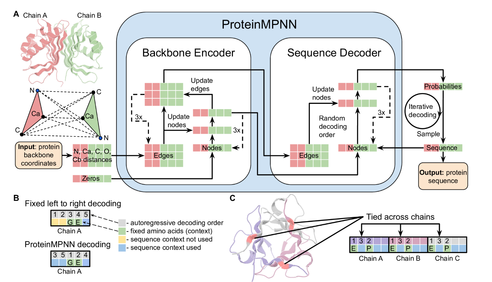
A)使用消息传递神经网络(Encoder)对N、Ca、C、O和虚拟Cb之间的距离进行编码和处理,以获得图节点和边缘特征。编码的特征与部分序列一起用于以随机解码顺序迭代生成氨基酸。(B)固定的从左到右解码不能对前面的位置(黄色)使用序列上下文(绿色),而使用随机解码顺序训练的模型可以在推理过程中使用任意解码顺序。可以选择解码顺序,以便首先解码固定上下文。 (C) 链内和链之间的残基位置可以连接在一起,从而实现对称、重复蛋白质和多状态设计。在本例中,同源三聚体被设计为不同链中位置的耦合。对并列位置的预测 logit 进行平均,以获得从中采样氨基酸的单一概率分布。
通过镜像对称的位点平均一下,采样同一个氨基酸
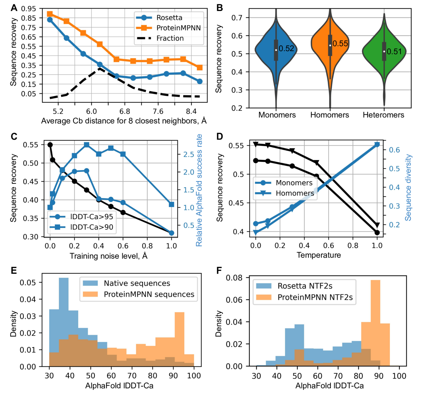
(A)ProteinMPNN比Rosetta具有更高的天然序列回收率。8个最近邻居的平均Cb距离(x轴)报告恢复情况,左侧恢复位置最多,右侧暴露较多; ProteinMPNN 在所有恢复级别都优于 Rosetta。ProteinMPNN 的平均序列恢复率为 52.4%,而 Rosetta 的平均序列恢复率为 32.9%。(B)ProteinMPNN对单体、同源寡聚物和异源寡聚物具有类似的高序列恢复率;小提琴图适用于 690 个单体、732 个同源体、98 个异构体。(C)序列恢复(黑色)和相对AlphaFold成功率(蓝色)作为训练噪声水平的函数。对于较高准确度的预测(圆圈),较小的噪声量是最佳的(1.0 对应于 1.8% 的成功率),而为了在较低的准确度截止值(正方形)下最大限度地提高预测成功率,使用更多噪声训练的模型更好(1.0 对应于 6.7% 的成功率)。(D)序列恢复和多样性随采样温度的变化。与使用无多序列信息的原始天然序列相比,使用 ProteinMPNN 重新设计天然蛋白质骨架可显着提高 AphaFold 预测准确性。在这两种情况下都输入了单个序列(设计的或天然的)。(F) 对先前 Rosetta 设计的 NTF2 折叠蛋白(总共 3,000 个主链)进行 ProteinMPNN 重新设计,从而显着提高了 AlphaFold 单序列预测精度。
使用主链噪声进行训练可提高蛋白质设计的模型性能
由于蛋白质表达、溶解度和功能的序列决定因素尚不完全清楚,因此在大多数蛋白质设计应用中,需要通过实验测试多个设计的序列。我们发现,通过在较高温度下进行推理,MPNN生成的序列多样性可以显着增加,平均序列回收率仅下降很小(图2D)。我们还发现,源自ProteinMPNN的序列质量测量,即给定结构的序列的平均对数概率,与在一定温度范围内的天然序列恢复率密切相关(图S3A),从而能够对序列进行快速排名以进行实验表征的选择。
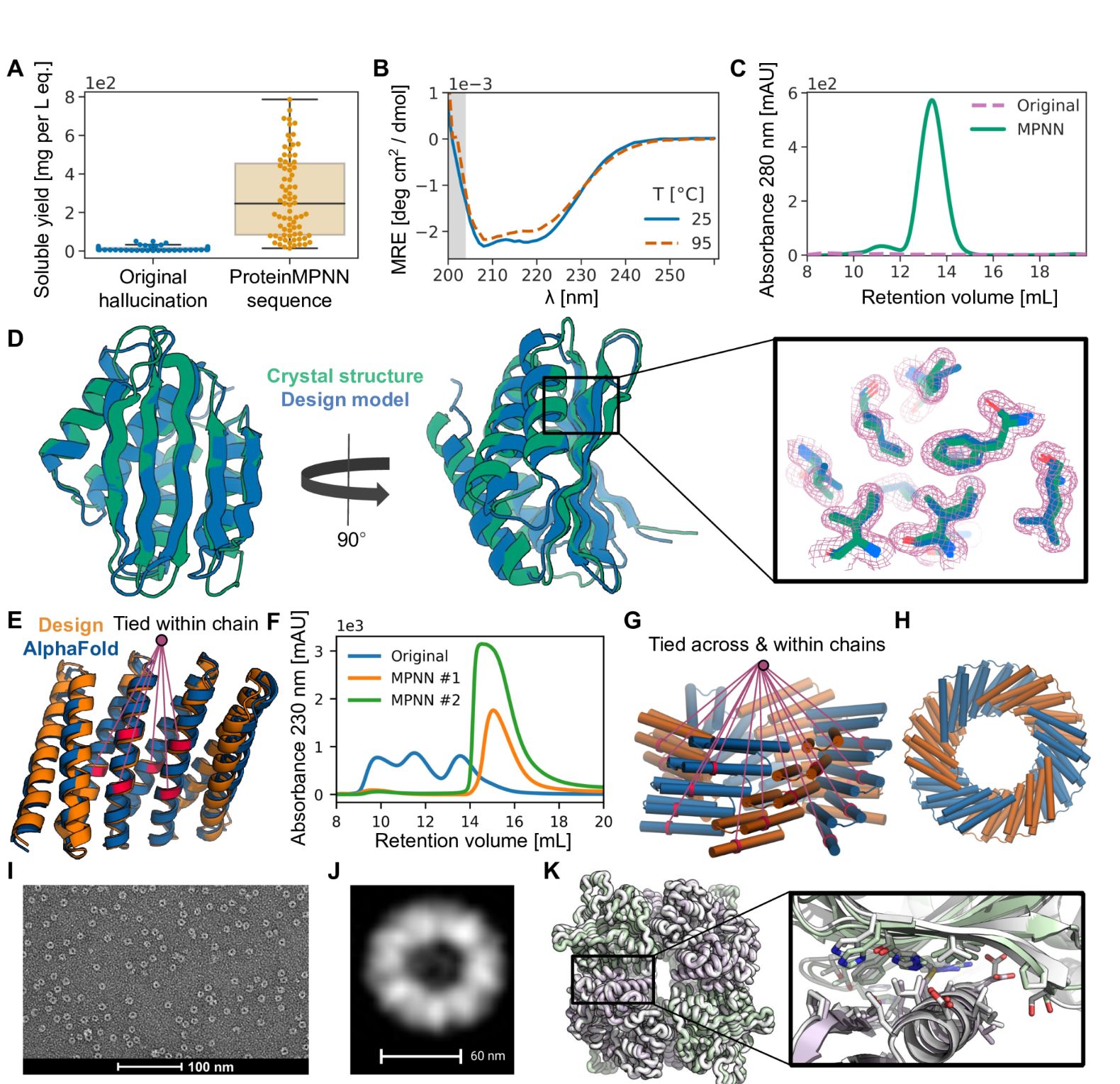
(A)一组AlphaFold幻觉单体和同源寡聚体(蓝色)以及使用ProteinMPNN(橙色)设计序列的同一组骨架的可溶性蛋白表达的比较,N=129。从镍-NTA纯化蛋白质的大小排除痕迹下的整合区域获得的大肠杆菌表达后的总可溶性蛋白质产量比ProteinMPNN拯救后原始序列的几乎不溶的蛋白质显着增加(1 L培养当量的中位产量:分别为9和247 mg)。(B)、(C)、(D) 单体幻觉的深入表征以及从 A 中的集合中拯救相应的 ProteinMPNN。与A中的几乎所有设计一样,设计模型的序列和结构相似性与PDB非常低(使用HHblits的UniRef100的E值=2.8,PDB的TM分数=0.56)。(B)ProteinMPNN拯救设计具有高热稳定性,与25 °C相比,在95 °C下圆二色性曲线几乎不变。 (C)与ProteinMPNN序列设计叠加的失败原始设计的尺寸排阻(SEC)曲线,在预期保留体积下具有明显的单分散峰。(D)ProteinMPNN(8CYK)设计的晶体结构与设计模型几乎相同(130个残基为2.35 RMSD),更多信息见图S5。右图显示了电子密度、绿色晶体侧链和蓝色 AlphaFold 侧链的模型侧链。(E)、(F)由完美重复的结构和序列单元(DHR82)制成的Rosetta设计的蛋白质MPNN救援。在 ProteinMPNN 序列推断期间,重复单元中相应位置的残基被绑定。(E)骨架设计模型和MPNN重新设计的序列AlphaFold模型,其连接残基由线表示(232个残基的~1.2Å误差)。(F)IMAC纯化的原始Rosetta设计和两个ProteinMPNN重新设计的SEC曲线。(G)、(H) 在链内和链之间的 ProteinMPNN 序列推断过程中连接残基,以强制执行重复蛋白质和循环对称性。(G)设计模型侧视图。一组捆绑的残基以红色显示。(H) 设计模型自上而下的视图。(I)纯化设计的负染色电子显微照片。(J) 来自 I 的图像的类平均值与 H 中的自上而下视图非常匹配。(K) 通过 ProteinMPNN 界面设计拯救失败的双组分 Rosetta 四面体纳米颗粒设计 T33-27 (13)。在 ProteinMPNN 救援后,纳米颗粒很容易组装,产量很高,晶体结构(灰色)与设计模型(绿色/紫色)几乎相同(在形成 ProteinMPNN 救援界面的两个完整的不对称单元上,主链 RMSD 为 1.2 Å)。
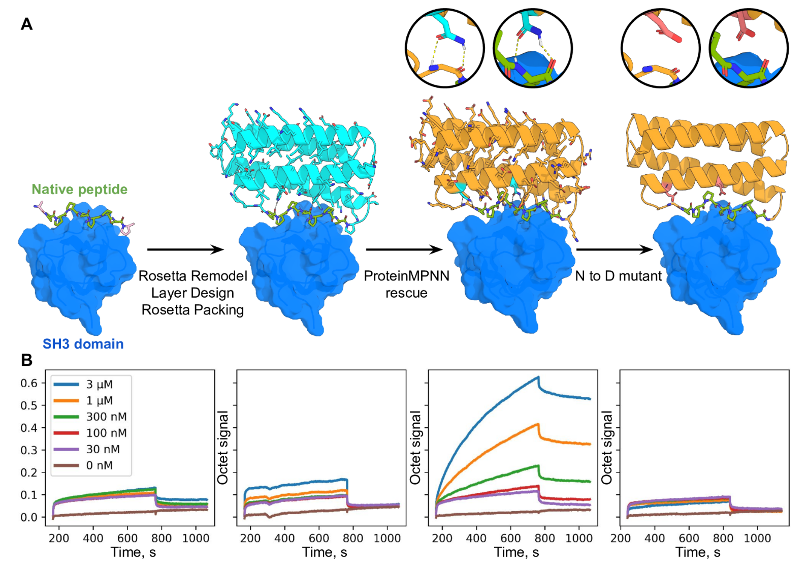
最后还评估了 ProteinMPNN 使用 Rosetta 挽救以前失败的新蛋白质功能设计的能力。
ProteinMPNN 在很短的时间内解决了序列设计问题(对于 100 个残基蛋白质,单个 CPU 为 1.2 秒,而单个 CPU 上为 258.8 秒),Rosetta 等基于物理的方法执行大规模侧链堆积计算,在天然骨架上实现了更高的蛋白质序列恢复率(52.4% 对 32.9%),最重要的是, 挽救了以前使用 Rosetta 或 AlphaFold 进行蛋白质单体、组装体和蛋白质-蛋白质界面的失败设计。以前已经开发了机器学习序列设计方法 (1-6),特别是前面描述的 ProteinMPNN 所基于的消息传递方法,但专注于单体设计问题,实现较低的天然序列恢复率,并且除了 TIM 桶设计研究 (6) 尚未使用晶体学和冷冻电镜进行广泛验证来评估设计准确性。虽然结构预测方法可以纯粹在计算机中进行评估,但蛋白质设计方法并非如此:计算机指标(例如天然序列回收)对晶体学分辨率非常敏感(图 S3 B、C),并且可能与适当的折叠(即使是单个残基替换,同时导致整体序列回收率变化很小), 可以阻挡折叠);就像语言翻译的准确性最终必须由人类用户评估一样,序列设计方法的最终测试是实验表征。
与 Rosetta 和其他基于物理的方法不同,ProteinMPNN 不需要专家定制来应对特定的设计挑战,因此它应该使蛋白质设计更广泛地可访问。这种鲁棒性反映了序列设计问题构建方式的根本差异。在传统的基于物理的方法中,序列设计映射到识别其最低能态是所需结构的氨基酸序列的问题。然而,这在计算上是棘手的,因为它需要所有可能结构的计算能量,包括不需要的寡聚态和聚集态; 相反,Rosetta 和其他方法作为代理,为给定的主链结构搜索最低能量序列,并且在第二步中需要进行结构预测计算,以确认没有其他结构中该序列的能量仍然较低。由于实际设计目标与显式优化的内容之间缺乏一致性,因此可能需要大量的定制才能生成实际折叠的序列;例如,在 Rosetta 设计计算中,疏水氨基酸通常会受到蛋白质表面的限制,因为它们可以稳定不需要的多聚体状态,并且在蛋白质表面和核心之间的边界区域,对于应应用此类限制的程度可能存在相当大的模糊性。 虽然深度学习方法缺乏 Rosetta 等方法的物理透明度,但它们经过直接训练,可以在 PDB 中的所有示例中找到最可能的蛋白质主链氨基酸,因此不会出现这种歧义,使序列设计更加稳健,并且更少依赖人类专家的判断。
ProteinMPNN 的实验设计成功率高,加上计算效率高、几乎适用于任何蛋白质序列设计问题以及无需定制,使其成为蛋白质设计研究所蛋白质序列设计的标准方法,我们预计它将在整个社区中迅速采用。如随附的论文(Wicky 等人)所示,ProteinMPNN 设计还具有更高的结晶倾向,极大地促进了设计蛋白质的结构测定。观察到,ProteinMPNN 生成的序列预计比原始天然序列更自信、更准确地折叠到天然蛋白质主链(在这两种情况下都使用单序列信息),这表明 ProteinMPNN 可能在改善重组表达的天然蛋白质的表达和稳定性方面具有广泛用途(功能所需的残基显然必须保持固定)。我们目前正在将 ProteinMPNN 扩展到蛋白质核酸设计和蛋白质小分子设计,这将进一步提高其实用性。
Methods
训练数据
对于表 1 中介绍的单链实验,我们使用了基于 CATH 4.2 40% 非冗余蛋白质集的数据集 (1, 7)。我们按照(1)中描述的设置训练模型,即使用原始Transformer论文(20)的学习率计划和初始化,10%的辍学率(21),10%的标签平滑率(22),具有6000个token的批量大小,使用Ca-Ca距离将图稀疏性设置为30个最近邻。
损失函数和优化
我们使用负对数似然,标签平滑率为 10% (22) 来计算损失(不使用标签平滑也很有效)。负概率的总和比对数概率的平均值效果要好得多。训练损失由损失平均值 = 总和(损失 * 掩码)/ 2000 定义,其中 2000 是根据经验选择的,损失(每个标记的分类交叉熵)和掩码具有形状 [批次,蛋白质长度]。为了进行优化,我们使用了 Adam,beta1 = 0.9,beta2 = 0.98,epsilon= 10−9,以及 (20) 中描述的学习率计划。在单个 NVIDIA A100 GPU 上使用 pytorch (24)、10k 令牌的批量大小、自动混合精度和梯度检查点训练模型。作为优化器步骤函数的训练和验证损失(困惑度)如图 3D 所示。验证损失在大约 150k 优化器步骤后收敛,这是来自 23,358 个 PDB 集群的大约 100 个动态采样训练数据的 epoch。
模型架构
| 模块 | 作用 | 对应论文描述 | 输入/输出维度 |
|---|---|---|---|
| Featurize() | 将蛋白结构坐标转换为模型输入特征(节点、边、掩码等) | “Graph construction from backbone coordinates” | 输出 (X, S, mask, chain_M, residue_idx, ...) |
| ProteinFeatures | 从坐标生成节点和边的几何特征,包括 RBF、相对位置、链信息 | “Feature construction and geometric encoding” | 输入 (X[B,L,4,3]) → 输出边特征 E[B,L,K,128] |
| Encoder (EncLayer × 3) | 信息聚合层,对结构图做 message passing | “Structure encoder” | 输入 (h_V[B,L,128], h_E[B,L,K,128]) |
| Decoder (DecLayer × 3) | 自回归解码层,从掩码残基生成氨基酸分布 | “Autoregressive sequence decoder” | 输入 (h_V, h_E, h_S) → 输出 log_probs[B,L,21] |
| Output Layer (W_out) | 输出每个位置的氨基酸 logits | “Logits for amino acid types” | [B, L, 21] |
- Featurize(batch)
| 名称 | 形状 | 含义 |
|---|---|---|
X |
[B, L, 4, 3] |
每个残基的原子坐标(N, CA, C, O) |
S |
[B, L] |
氨基酸种类(整数索引) |
mask |
[B, L] |
1 表示有效残基 |
chain_M |
[B, L] |
1 表示要预测的残基(masked chain) |
residue_idx |
[B, L] |
全局残基索引(跨链连续编号) |
chain_encoding_all |
[B, L] |
链 ID(整数编码) |
- 图构建与几何编码:
ProteinFeatures
输入:X (B,L,4,3)
输出:
E:[B, L, K, edge_dim=128]E_idx:[B, L, K]邻居索引(top-K 最近邻)
核心步骤:
- 计算 Cα–Cα 距离矩阵;
- 选取每个残基的 top-K 近邻;
- 计算 25 种不同原子对之间的径向基函数(RBF)特征(例如 N–N, C–C, O–O, Cα–Cb, 等);
- 每种原子对产生
num_rbf=16维 → 总计25×16 = 400;
- 每种原子对产生
- 计算残基的相对顺序偏移(offset embedding, 约 65 维);
- 拼接后通过线性层 →
edge_features=128; - LayerNorm。
输出的边特征 E 就是图的连接权重,用于 message passing。
没有提供侧链Cb原子坐标,通过几何构造公式(基于理想键长、键角、二面角)
构建局部邻域,包括计算距离矩阵,选取k-neighbor个邻居,得到
E_idx:每个残基的邻居索引
D_neighbors:对应距离
构造5*5=25种径向基函数,每对距离16维度,一共16*25=400维度
再进行相对位置与链信息编码,concat,layernorm
这样就得到和h_E,h_V是初始化为零向量
- Encoder(结构编码器)
输入:
节点初始特征
h_V = zeros([B,L,128])边特征线性映射
h_E = W_e(E)→[B,L,K,128]输入:
- 节点:
h_V [B,L,128] - 边:
h_E [B,L,K,128]
- 节点:
拼接后:
h_EV = concat(h_V_i, h_E_ij, h_V_j)→[B,L,K,256]线性层序列:
W1 → W2 → W3(每层输出 128)残差 + LayerNorm + Dropout
FeedForward (128→512→128)
输出:更新后的
h_V, h_E,形状不变[B,L,128],[B,L,K,128]Decoder(自回归解码器)
输入:
- 结构编码后的
h_V(来自 encoder) - 边特征
h_E - 已知序列嵌入
h_S = Embedding(S)→[B,L,128]
- 结构编码后的
流程:
拼接邻居节点和边:
h_ES = cat_neighbors_nodes(h_S, h_E, E_idx)→[B,L,K,256]生成自回归掩码:
- 随机打乱 masked 残基顺序;
- 构造前向(mask_fw)和后向(mask_bw)掩码;
结合结构编码结果:
h_EXV_encoder_fw = mask_fw * h_EXV_encoder多层解码:
1
2
3
4
for i in range(3):
h_ESV = cat_neighbors_nodes(h_V, h_ES, E_idx)
h_ESV = mask_bw * h_ESV + h_EXV_encoder_fw
h_V = DecLayer(h_V, h_ESV)输出 logits:
logits = W_out(h_V)→[B, L, 21]
log_probs = log_softmax(logits)
内部结构:
与 EncLayer 类似,但更简单:
只更新节点向量;
输入
[B,L,128],输出[B,L,128];内含 3 个线性层 + GELU + 残差 + LayerNorm;
FeedForward (128→512→128)。
输出层与损失
输出:
log_probs:[B, L, 21]
损失函数:
loss_nll: 负对数似然 NLL(每个残基的氨基酸预测概率)loss_smoothed: 带 label smoothing 的版本
| 名称 | 形状 | 类型 | 含义 |
|---|---|---|---|
X |
[B, L_max, 4, 3] |
float tensor | 每个残基 N,CA,C,O 的 xyz;pad 部分被置 0,但 mask 标记为 0 |
S |
[B, L_max] |
long tensor | 序列标签(整型索引),pad 为 0 |
mask |
[B, L_max] |
float tensor | 1.0 表示该位置有真实坐标(可用于计算),0.0 表示 pad |
lengths |
[B] |
numpy int | 每个样本的真实长度 |
chain_M |
[B, L_max] |
float tensor | 1.0 = 该位置需要被模型预测(masked),0.0 = visible(已知) |
residue_idx |
[B, L_max] |
long tensor | 全局残基索引(含链间跳跃),用于构造相对位置/offset |
mask_self |
[B, L_max, L_max] |
float tensor | 0 表示同链内部(不算作 interface),1 表示可能的跨链交互(用于 interface loss) |
chain_encoding_all |
[B, L_max] |
long tensor | 链编号(整数),用于 chain-aware embedding/特征 |
N, CA, C, O 四原子:这些主链原子能完整表示主链几何(主链走向与局部平面),后续网络会基于这些构建 Cβ(代码在 ProteinFeatures 中用叉积估计虚拟 Cβ)并计算多种原子对的 RBF 特征。把原子顺序固定(N,CA,C,O)确保后面的几何计算一致。
用 NaN 做 padding:方便直接通过 isfinite 检测有效位置然后再统一填 0,避免对后续几何计算产生不合理偏移。
residue_idx 带链跳跃:在计算相对位置(offset)时能够区分“同链但不同位置”与“跨链”场景(特别对对称/多链任务很重要)。
chain_M 与随机链顺序:随机打乱链顺序 + chain mask 可以训练模型去适应不同链排列与部分已知/部分未知的场景(即 order-agnostic decoding)。
mask_self:为 interface 专门做的掩码,后面计算 interface loss 时通常只想考虑跨链相互作用,不希望把同链内部也计入。
== 模型结构信息 ==
模块: features, 类型: ProteinFeatures
模块: W_e, 类型: Linear #编码结构特征到Encoder
模块: W_s, 类型: Embedding #编码序列特征到Decoder
模块: encoder_layers, 类型: ModuleList
模块: decoder_layers, 类型: ModuleList
模块: W_out, 类型: Linear
== 可训练参数详情 ==
可训练: features.embeddings.linear.weight, 形状: torch.Size([16, 66]), 参数量: 1,056
可训练: features.embeddings.linear.bias, 形状: torch.Size([16]), 参数量: 16
可训练: features.edge_embedding.weight, 形状: torch.Size([128, 416]), 参数量: 53,248
可训练: features.norm_edges.weight, 形状: torch.Size([128]), 参数量: 128
可训练: features.norm_edges.bias, 形状: torch.Size([128]), 参数量: 128
可训练: W_e.weight, 形状: torch.Size([128, 128]), 参数量: 16,384
可训练: W_e.bias, 形状: torch.Size([128]), 参数量: 128
可训练: W_s.weight, 形状: torch.Size([21, 128]), 参数量: 2,688
可训练: encoder_layers.0.norm1.weight, 形状: torch.Size([128]), 参数量: 128
可训练: encoder_layers.0.norm1.bias, 形状: torch.Size([128]), 参数量: 128
可训练: encoder_layers.0.norm2.weight, 形状: torch.Size([128]), 参数量: 128
可训练: encoder_layers.0.norm2.bias, 形状: torch.Size([128]), 参数量: 128
可训练: encoder_layers.0.norm3.weight, 形状: torch.Size([128]), 参数量: 128
可训练: encoder_layers.0.norm3.bias, 形状: torch.Size([128]), 参数量: 128
可训练: encoder_layers.0.W1.weight, 形状: torch.Size([128, 384]), 参数量: 49,152
可训练: encoder_layers.0.W1.bias, 形状: torch.Size([128]), 参数量: 128
可训练: encoder_layers.0.W2.weight, 形状: torch.Size([128, 128]), 参数量: 16,384
可训练: encoder_layers.0.W2.bias, 形状: torch.Size([128]), 参数量: 128
可训练: encoder_layers.0.W3.weight, 形状: torch.Size([128, 128]), 参数量: 16,384
可训练: encoder_layers.0.W3.bias, 形状: torch.Size([128]), 参数量: 128
可训练: encoder_layers.0.W11.weight, 形状: torch.Size([128, 384]), 参数量: 49,152
可训练: encoder_layers.0.W11.bias, 形状: torch.Size([128]), 参数量: 128
可训练: encoder_layers.0.W12.weight, 形状: torch.Size([128, 128]), 参数量: 16,384
可训练: encoder_layers.0.W12.bias, 形状: torch.Size([128]), 参数量: 128
可训练: encoder_layers.0.W13.weight, 形状: torch.Size([128, 128]), 参数量: 16,384
可训练: encoder_layers.0.W13.bias, 形状: torch.Size([128]), 参数量: 128
可训练: encoder_layers.0.dense.W_in.weight, 形状: torch.Size([512, 128]), 参数量: 65,536
可训练: encoder_layers.0.dense.W_in.bias, 形状: torch.Size([512]), 参数量: 512
可训练: encoder_layers.0.dense.W_out.weight, 形状: torch.Size([128, 512]), 参数量: 65,536
可训练: encoder_layers.0.dense.W_out.bias, 形状: torch.Size([128]), 参数量: 128
可训练: encoder_layers.1.norm1.weight, 形状: torch.Size([128]), 参数量: 128
可训练: encoder_layers.1.norm1.bias, 形状: torch.Size([128]), 参数量: 128
可训练: encoder_layers.1.norm2.weight, 形状: torch.Size([128]), 参数量: 128
可训练: encoder_layers.1.norm2.bias, 形状: torch.Size([128]), 参数量: 128
可训练: encoder_layers.1.norm3.weight, 形状: torch.Size([128]), 参数量: 128
可训练: encoder_layers.1.norm3.bias, 形状: torch.Size([128]), 参数量: 128
可训练: encoder_layers.1.W1.weight, 形状: torch.Size([128, 384]), 参数量: 49,152
可训练: encoder_layers.1.W1.bias, 形状: torch.Size([128]), 参数量: 128
可训练: encoder_layers.1.W2.weight, 形状: torch.Size([128, 128]), 参数量: 16,384
可训练: encoder_layers.1.W2.bias, 形状: torch.Size([128]), 参数量: 128
可训练: encoder_layers.1.W3.weight, 形状: torch.Size([128, 128]), 参数量: 16,384
可训练: encoder_layers.1.W3.bias, 形状: torch.Size([128]), 参数量: 128
可训练: encoder_layers.1.W11.weight, 形状: torch.Size([128, 384]), 参数量: 49,152
可训练: encoder_layers.1.W11.bias, 形状: torch.Size([128]), 参数量: 128
可训练: encoder_layers.1.W12.weight, 形状: torch.Size([128, 128]), 参数量: 16,384
可训练: encoder_layers.1.W12.bias, 形状: torch.Size([128]), 参数量: 128
可训练: encoder_layers.1.W13.weight, 形状: torch.Size([128, 128]), 参数量: 16,384
可训练: encoder_layers.1.W13.bias, 形状: torch.Size([128]), 参数量: 128
可训练: encoder_layers.1.dense.W_in.weight, 形状: torch.Size([512, 128]), 参数量: 65,536
可训练: encoder_layers.1.dense.W_in.bias, 形状: torch.Size([512]), 参数量: 512
可训练: encoder_layers.1.dense.W_out.weight, 形状: torch.Size([128, 512]), 参数量: 65,536
可训练: encoder_layers.1.dense.W_out.bias, 形状: torch.Size([128]), 参数量: 128
可训练: encoder_layers.2.norm1.weight, 形状: torch.Size([128]), 参数量: 128
可训练: encoder_layers.2.norm1.bias, 形状: torch.Size([128]), 参数量: 128
可训练: encoder_layers.2.norm2.weight, 形状: torch.Size([128]), 参数量: 128
可训练: encoder_layers.2.norm2.bias, 形状: torch.Size([128]), 参数量: 128
可训练: encoder_layers.2.norm3.weight, 形状: torch.Size([128]), 参数量: 128
可训练: encoder_layers.2.norm3.bias, 形状: torch.Size([128]), 参数量: 128
可训练: encoder_layers.2.W1.weight, 形状: torch.Size([128, 384]), 参数量: 49,152
可训练: encoder_layers.2.W1.bias, 形状: torch.Size([128]), 参数量: 128
可训练: encoder_layers.2.W2.weight, 形状: torch.Size([128, 128]), 参数量: 16,384
可训练: encoder_layers.2.W2.bias, 形状: torch.Size([128]), 参数量: 128
可训练: encoder_layers.2.W3.weight, 形状: torch.Size([128, 128]), 参数量: 16,384
可训练: encoder_layers.2.W3.bias, 形状: torch.Size([128]), 参数量: 128
可训练: encoder_layers.2.W11.weight, 形状: torch.Size([128, 384]), 参数量: 49,152
可训练: encoder_layers.2.W11.bias, 形状: torch.Size([128]), 参数量: 128
可训练: encoder_layers.2.W12.weight, 形状: torch.Size([128, 128]), 参数量: 16,384
可训练: encoder_layers.2.W12.bias, 形状: torch.Size([128]), 参数量: 128
可训练: encoder_layers.2.W13.weight, 形状: torch.Size([128, 128]), 参数量: 16,384
可训练: encoder_layers.2.W13.bias, 形状: torch.Size([128]), 参数量: 128
可训练: encoder_layers.2.dense.W_in.weight, 形状: torch.Size([512, 128]), 参数量: 65,536
可训练: encoder_layers.2.dense.W_in.bias, 形状: torch.Size([512]), 参数量: 512
可训练: encoder_layers.2.dense.W_out.weight, 形状: torch.Size([128, 512]), 参数量: 65,536
可训练: encoder_layers.2.dense.W_out.bias, 形状: torch.Size([128]), 参数量: 128
可训练: decoder_layers.0.norm1.weight, 形状: torch.Size([128]), 参数量: 128
可训练: decoder_layers.0.norm1.bias, 形状: torch.Size([128]), 参数量: 128
可训练: decoder_layers.0.norm2.weight, 形状: torch.Size([128]), 参数量: 128
可训练: decoder_layers.0.norm2.bias, 形状: torch.Size([128]), 参数量: 128
可训练: decoder_layers.0.W1.weight, 形状: torch.Size([128, 512]), 参数量: 65,536
可训练: decoder_layers.0.W1.bias, 形状: torch.Size([128]), 参数量: 128
可训练: decoder_layers.0.W2.weight, 形状: torch.Size([128, 128]), 参数量: 16,384
可训练: decoder_layers.0.W2.bias, 形状: torch.Size([128]), 参数量: 128
可训练: decoder_layers.0.W3.weight, 形状: torch.Size([128, 128]), 参数量: 16,384
可训练: decoder_layers.0.W3.bias, 形状: torch.Size([128]), 参数量: 128
可训练: decoder_layers.0.dense.W_in.weight, 形状: torch.Size([512, 128]), 参数量: 65,536
可训练: decoder_layers.0.dense.W_in.bias, 形状: torch.Size([512]), 参数量: 512
可训练: decoder_layers.0.dense.W_out.weight, 形状: torch.Size([128, 512]), 参数量: 65,536
可训练: decoder_layers.0.dense.W_out.bias, 形状: torch.Size([128]), 参数量: 128
可训练: decoder_layers.1.norm1.weight, 形状: torch.Size([128]), 参数量: 128
可训练: decoder_layers.1.norm1.bias, 形状: torch.Size([128]), 参数量: 128
可训练: decoder_layers.1.norm2.weight, 形状: torch.Size([128]), 参数量: 128
可训练: decoder_layers.1.norm2.bias, 形状: torch.Size([128]), 参数量: 128
可训练: decoder_layers.1.W1.weight, 形状: torch.Size([128, 512]), 参数量: 65,536
可训练: decoder_layers.1.W1.bias, 形状: torch.Size([128]), 参数量: 128
可训练: decoder_layers.1.W2.weight, 形状: torch.Size([128, 128]), 参数量: 16,384
可训练: decoder_layers.1.W2.bias, 形状: torch.Size([128]), 参数量: 128
可训练: decoder_layers.1.W3.weight, 形状: torch.Size([128, 128]), 参数量: 16,384
可训练: decoder_layers.1.W3.bias, 形状: torch.Size([128]), 参数量: 128
可训练: decoder_layers.1.dense.W_in.weight, 形状: torch.Size([512, 128]), 参数量: 65,536
可训练: decoder_layers.1.dense.W_in.bias, 形状: torch.Size([512]), 参数量: 512
可训练: decoder_layers.1.dense.W_out.weight, 形状: torch.Size([128, 512]), 参数量: 65,536
可训练: decoder_layers.1.dense.W_out.bias, 形状: torch.Size([128]), 参数量: 128
可训练: decoder_layers.2.norm1.weight, 形状: torch.Size([128]), 参数量: 128
可训练: decoder_layers.2.norm1.bias, 形状: torch.Size([128]), 参数量: 128
可训练: decoder_layers.2.norm2.weight, 形状: torch.Size([128]), 参数量: 128
可训练: decoder_layers.2.norm2.bias, 形状: torch.Size([128]), 参数量: 128
可训练: decoder_layers.2.W1.weight, 形状: torch.Size([128, 512]), 参数量: 65,536
可训练: decoder_layers.2.W1.bias, 形状: torch.Size([128]), 参数量: 128
可训练: decoder_layers.2.W2.weight, 形状: torch.Size([128, 128]), 参数量: 16,384
可训练: decoder_layers.2.W2.bias, 形状: torch.Size([128]), 参数量: 128
可训练: decoder_layers.2.W3.weight, 形状: torch.Size([128, 128]), 参数量: 16,384
可训练: decoder_layers.2.W3.bias, 形状: torch.Size([128]), 参数量: 128
可训练: decoder_layers.2.dense.W_in.weight, 形状: torch.Size([512, 128]), 参数量: 65,536
可训练: decoder_layers.2.dense.W_in.bias, 形状: torch.Size([512]), 参数量: 512
可训练: decoder_layers.2.dense.W_out.weight, 形状: torch.Size([128, 512]), 参数量: 65,536
可训练: decoder_layers.2.dense.W_out.bias, 形状: torch.Size([128]), 参数量: 128
可训练: W_out.weight, 形状: torch.Size([21, 128]), 参数量: 2,688
可训练: W_out.bias, 形状: torch.Size([21]), 参数量: 21